Using the Percentage Format in Table Cells
Use the percentage format to display numeric values followed by the percent
symbol (%).
If the value is used in a formula, its decimal number version is used. For example, a
value that displays as 3.00% is used as 0.03 in a formula.
If you type 3% in a cell formatted using the automatic format and then apply the
percentage format to the cell, the value displayed is 3%. However, if you type 3 in a cell
formatted using the automatic format and then apply the percentage format to the
cell, the value displayed is 300%.
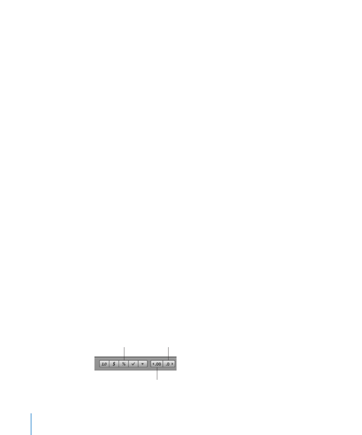
To define a percentage format that displays two decimal places, a thousands
separator, and negative numbers with the negative symbol, select one or more cells
and then click the Percentage Format button in the format bar. Use the Decrease
Decimal Places and Increase Decimal Places buttons located nearby to change the
number of decimal places.
Increase Decimal
Places button
Decrease Decimal
Places button
Percentage
Format button
94
Chapter 4
Working with Table Cells

Chapter 4
Working with Table Cells
95
For more control over the percentage format, use the Cells inspector.
To define a percentage format using the Cells inspector:
1
Select the cell or cells.
2
Click Inspector in the toolbar, and then click the Cells inspector button.
3
Choose Percentage from the Cell Format pop-up menu.
4
To specify how many decimal places to display, use the Decimals field.
If a value contains more decimal places than you specify, the decimal value displayed
is rounded, not truncated. For example, if a cell is formatted to display two decimal
places, the value 3.456 is displayed as 3.46, not 3.45.
5
To specify how to display negative values, choose an entry from the pop-up menu
adjacent to the Decimals field.
6
To specify whether to use a thousands separator, select or deselect Thousands Separator.
If a cell you’re formatting already contains a value, the value is assumed to be a
decimal value, and it’s converted into a percentage. For example, 3 becomes 300%.